Supervised Single-View to 3D Objects

3D reconstruction from a single view is very similar to the process through which we recognize objects in the real world. When we look at a chair from one angle, we know it is a chair and can intuitively imagine what it would look like from other angles. It’s not like a chair viewed from one angle will look like an airplane from another angle. That being said, if you were determined to design an airplane that looks like a chair from a specific viewpoint, then everything in this post is inapplicable. 🤣

How is it Possible to Know the Depth from a Single View?

Deriving depth information from a single view is an ill-posed problem, meaning there are infinitely many possible solutions for reconstructing the 3D scene from a 2D image. This complexity arises because a single ray projected from the camera center to a pixel in the image can intersect with any point along its path, making the depth information inherently ambiguous without additional cues.

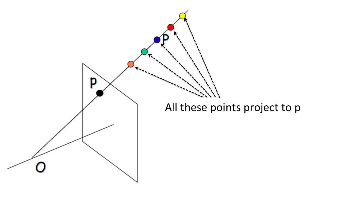
The image above is adapted from here.

Despite this being an ill-posed problem, it is still possible to infer depth from a single view by exploiting the regularities and cues present in the natural world. For instance, depth can be inferred from single images through cues such as occlusion (where one object blocks another), relative size (larger objects are perceived as closer), perspective (parallel lines appear to converge with distance), and shading/lighting.

Furthermore, we can train models to recognize patterns and learn these visual cues from extensive datasets where the true depth or shape information is known.

In this post, I will show how numerous images and objects’ 3D structures can be used to train a neural network to deduce a 3D shape from a single 2D image.

What Coordinate Systems Should We Predict 3D Models In?

Different coordinates systems serves different purposes in 3D world. Here, three coordinate systems related to this subject are brought up, each with different charateristics.

1. Camera Coordinate System: it is inherently aligned with our perspective. This system adjusts the coordinates of an object based on its movements or rotations relative to the camera. This means that any change in the object’s position or orientation directly alters its coordinates within this system. However, this approach has its limitations. It can introduce confusion between the actual shape of an object and its perceived location from the camera’s viewpoint. This overlap of shape and position uncertainties can make it challenging to accurately predict a 3D model’s shape.

   
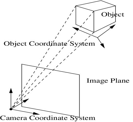
   Camera Coordinate System. The image is adapted from "Methods for Structure from Motion" by Henrik Aanæs.

2. View-aligned Object-centric Coordinate System: it centers inside the object, usually at the average location of its parts. This system decouples the object’s shape from its spatial position.

   What makes it “view-aligned” is that the object’s coordinates adjust based on where we’re looking from, ensuring that the object’s coordinates always relate directly to our viewpoint. This means that the object’s coordinates don’t change if we only vary the distance between the observer and the object along the direction from the camera to the object. A major limitation of this approach is that we need to generate a distinct 3D shape for each viewpoint of the object, complicating the model prediction process.

3. Object-centric “Canonical” Coordinate System: In this system, a “canonical” definition for axis orientation is established where the Y-axis points up, and the -Z-axis faces the front of the object. Defining the “front” of an object can sometimes be challenging and is often determined by convention or the dataset creator. This system helps in standardizing object representation across various observations. This system ensures uniform object representation across different viewpoints by keeping the object’s coordinates constant, regardless of its movement or rotation relative to the observer.

Visualizing coordinate systems:

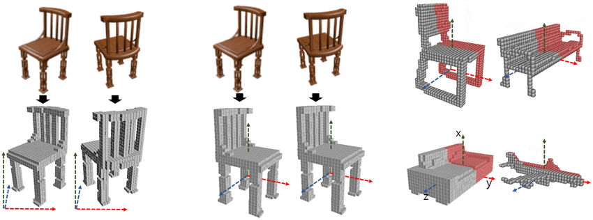
This visualization is adapted from "Sym3DNet: Symmetric 3D Prior Network for Single-View 3D Reconstruction."

The left image illustrates the view-aligned object-centric coordinate system (let’s pretend the coordinate system centered within a chair,) indicating how this system adapts to the viewer’s perspective.

The middle image depicts the object-centric canonical coordinate system, showcasing a method where the object’s orientation and position are standardized, irrespective of the viewer’s perspective.

The right image demonstrates that in the canonical view, all 3D shapes are uniformly aligned within the world’s 3D space, offering a consistent framework for object representation.

Visualizing ground truth w.r.t. the coordinate system:

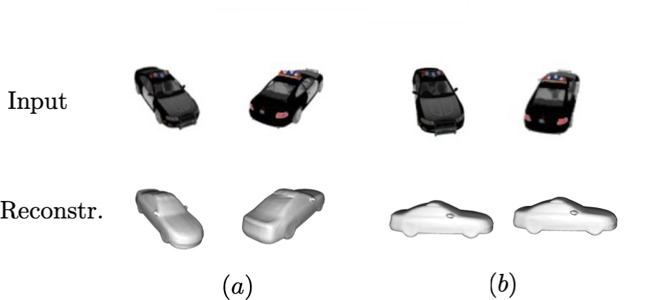
This visualization is adapted from "On the generalization of learning-based 3D reconstruction."

The image above shows that a view-aligned object-centric coordinate system dynamically adjusts the ground truth coordinate system to match the orientation of the input view. In contrast, an object-centric canonical coordinate system maintains the ground truth anchored to a canonical frame, unaffected by the perspective of 2D input view.

Now, the goal is clearly defined: given an object image view from an arbitrary angle, predict the object’s 3D shape in the object-centric canonical coordinate system. Predictions in the object-centric canonical coordinate system should be invariant to the observed viewpoint, ensuring consistent and accurate 3D models across different observations.

Dataset Visualization

In this project, I use the r2n2_shapenet_dataset, a synthetic dataset designed in structured environments. While synthetic data offers benefits such as ease of prototyping and testing, it also comes with its challenges. One significant issue is that synthetic data may favor artificial categories, leading to biases that do not accurately represent the diversity and variability found in real-life objects and environments.

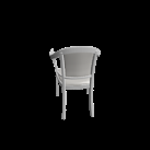
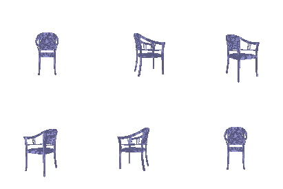
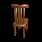
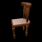
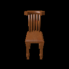
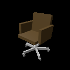
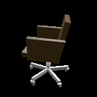
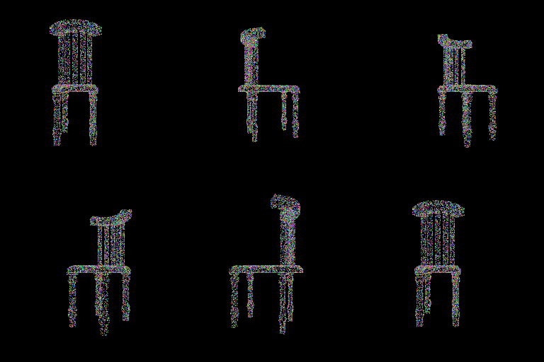
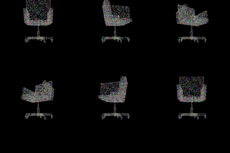
For each training example, the dataset provides up to 24 views of a chair image, along with mesh objects and voxels. It does not include point clouds; however, we can use sample_points_from_meshes() to generate point clouds from the ground truth meshes.

Below are examples of multiple views from three different chairs:

During the training phase, the data loader randomly selects one view for the input. An important observation is that all meshes’ vertices are positioned close to the origin, with their centers very near to (0, 0, 0) and scales within [-1, 1].

Building a Model to Predict 3D Shape from a Single 2D Image

Now, we are ready to build a model which can predict an object’s 3D shape from a single 2D image.

Calculating Loss Between Point Clouds

To evaluate the accuracy of our model’s predictions against the ground truth, we use the Chamfer distance for loss calculation between two point clouds. The Chamfer distance is defined as:

\[d_{\text{CD}}(S_1, S_2) = \frac{1}{|S_1|} \sum_{x \in S_1} \min_{y \in S_2} \|x - y\|^2 + \frac{1}{|S_2|} \sum_{y \in S_2} \min_{x \in S_1} \|x - y\|^2\]

The Chamfer distance calculates the mean squared distance between each point in one cloud to its nearest neighbor in the other cloud, and vice versa, effectively measuring the overall similarity between the two shapes.

With the help of knn_points from PyTorch3D, I implement the Chamfer distance as follow:

def chamfer_loss(point_cloud_src, point_cloud_tgt):
    # point_cloud_src, point_cloud_src: (batch, n_points, 3)

    k = 1  # the number of nearest neighbors
    # knn_points returns K-Nearest neighbors on point clouds.
    src_dists, _, _ = knn_points(point_cloud_src, point_cloud_tgt, K=k)
    tgt_dists, _, _ = knn_points(point_cloud_tgt, point_cloud_src, K=k)
    # src_dists, tgt_dists: (batch, n_points, k)

    return (src_dists.mean() + tgt_dists.mean()) / 2  # Calculate the mean distance.

Fitting a target 3D Point Cloud with a Random Point Cloud

To validate the correct implementation of chamfer_loss, we can fit a random point cloud to the target point cloud using chamfer_loss. Below is a simplified Python script showing this process:

n_points = 10000
pointclouds_source = torch.randn([1, n_points, 3], requires_grad=True)
optimizer = torch.optim.Adam([pointclouds_source], lr=1e-4)

for step in range(0, 50000):
    loss = chamfer_loss(pointclouds_source, pointclouds_groundtruth)
    optimizer.zero_grad()
    loss.backward()
    optimizer.step()

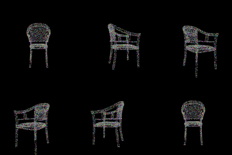
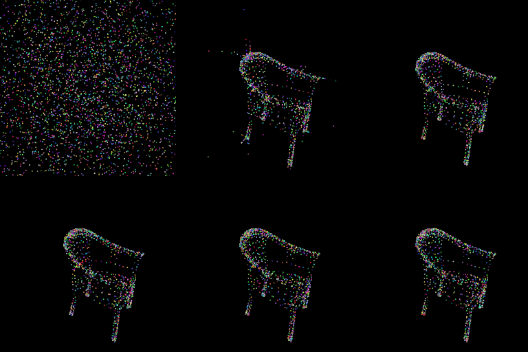
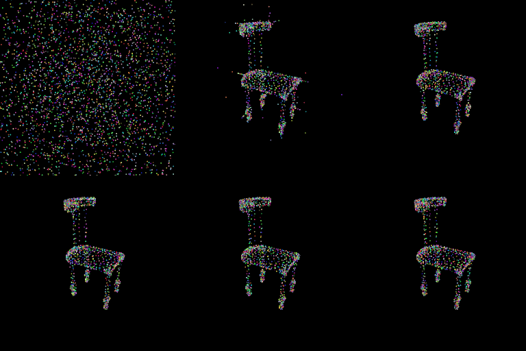
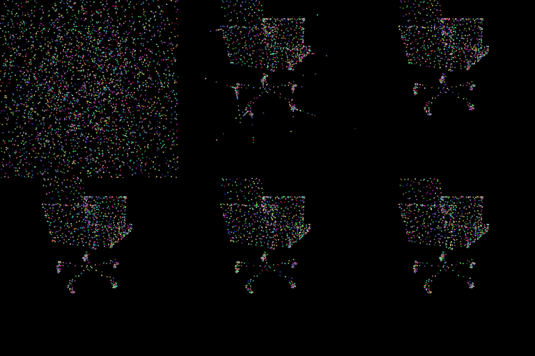
The following visualizations showcase the progressive alignment of the random point cloud towards the ground truth, as facilitated by minimizing the Chamfer distance through gradient descent:

Defining PointModel

The PointModel class, derived from torch.nn.Module, forms the backbone of our architecture, designed to transform 2D images into 3D point clouds. It is composed of two primary parts:

1. 2D Encoder: Transforms an image into a latent representation, capturing the essential features required for 3D reconstruction. I use a ResNet modoel from torchvision.models.
2. 3D Decoder: Converts the latent representation into a discrete 3D point clouds, where each point represents the location in the 3D world.

Below is the implementation of the PointModel:

class PointModel(nn.Module):
    def __init__(self, arch, n_points):
        super(PointModel, self).__init__()

        vision_model = torchvision_models.__dict__[arch](pretrained=True)
        self.encoder = torch.nn.Sequential(*(list(vision_model.children())[:-1]))
        self.normalize = transforms.Normalize(
            mean=[0.485, 0.456, 0.406], std=[0.229, 0.224, 0.225]
        )

        self.n_point = n_points

        encoder_out_size = 512
        # Encoder output: (batch, encoder_out_size)
        # Decoder output: (batch, n_points * 3)

        self.decoder = torch.nn.Sequential(
            torch.nn.Linear(encoder_out_size, 1024),
            torch.nn.ReLU(),
            torch.nn.Linear(1024, 2048),
            torch.nn.ReLU(),
            torch.nn.Linear(2048, n_points * 3),
            torch.nn.Tanh()
        )

    def forward(self, images, args):
        images_normalize = self.normalize(images.permute(0, 3, 1, 2))
        encoded_feat = self.encoder(images_normalize).squeeze(-1).squeeze(-1)  # (batch, encoder_out_size)
        pointclouds_pred = self.decoder(encoded_feat)
        return pointclouds_pred.view(-1, self.n_point, 3)

A few important aspects to note:

• The output size of the encoder varies depending on whether a resnet18 or resnet34 (512-vector) or a resnet50 (2048-vector) is used.
• I use the hyperbolic tangent (Tanh()) activation function in the final layer to ensure that every output point is constrained within the [-1, 1] range. I mention that the vertices of the mesh are within the [-1, 1] range in the previous section.

Evaluation Metrics

Given a point in the predicted point cloud, we calculate the distance between this point and its nearest point in the ground truth point cloud. If the distance falls below a predefined threshold, then we consider this point as a true positive. The criteria for categorizing points are as follows:

• True Positive (TP): A point in the predicted point cloud that is within a specified distance threshold of any point in the ground truth point cloud.
• False Positive (FP): A point in the predicted point cloud that is not within the threshold distance of any point in the ground truth point cloud.
• False Negative (FN): A point in the ground truth point cloud that is not within the threshold distance of any point in the predicted point cloud.

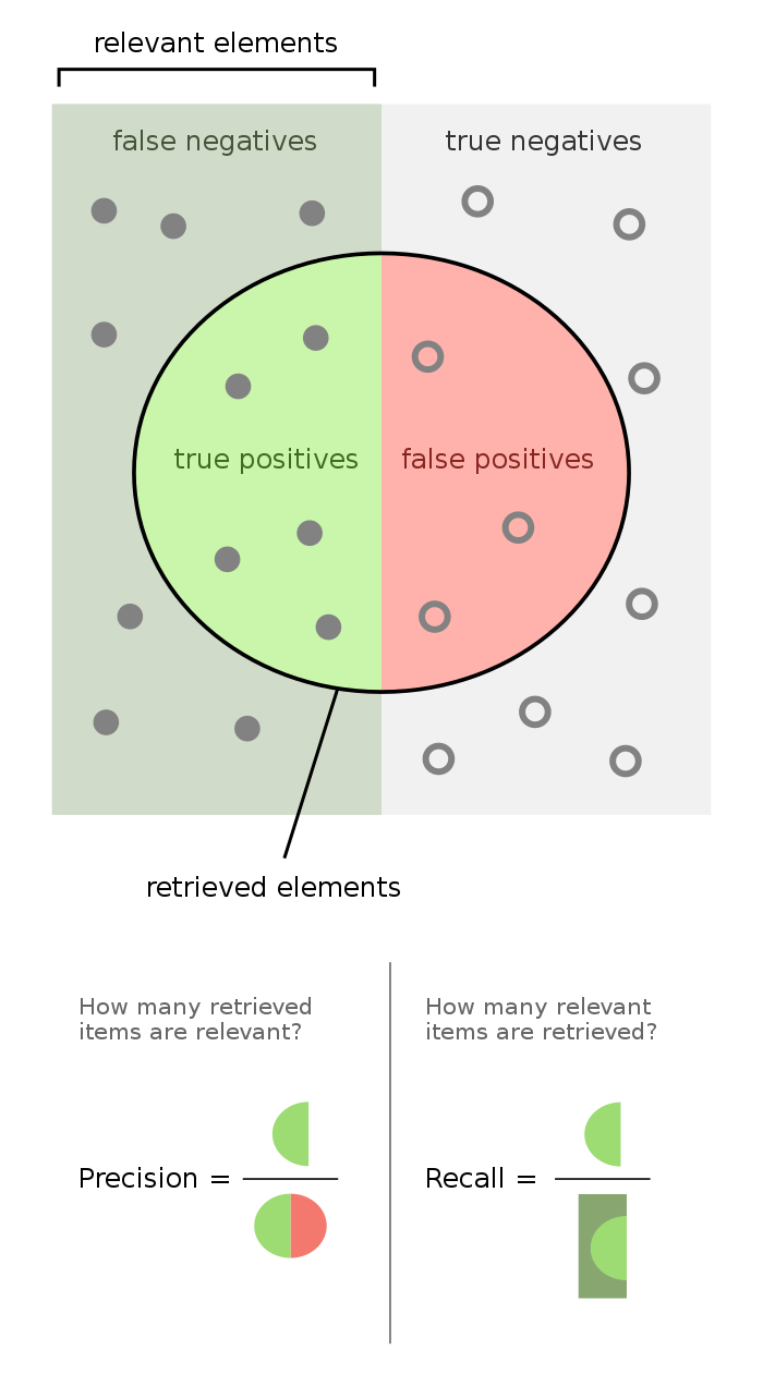
The image is adapted from Precision and Recall (Wikipedia).

The definitions of precision and recall are as follows:

• Precision measures the proportion of predicted points that are true positives out of all points predicted. $\text{Precision} = TP/(TP+FP)$
• Recall measures the proportion of true positives out of the points in the ground truth point cloud. $\text{Recall} = TP/(TP+FN)$
• F1 Score is the harmonic mean of precision and recall, providing a balance between them. $\text{F1 Score} = 2 * Precision * Recall / (Precision + Recall)$

Experimentation Results: Single View 2D Images to 3D Point Clouds

Preliminary experiments show the model can deduce 3D structures from single 2D images effectively. After using 10,000 points and conducting 100 epochs of training, the result is shown below.

Visual Results

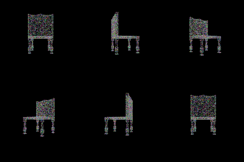
Ground truth point cloud.

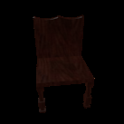
Single view image.

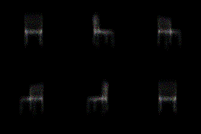
Predicted point cloud.

It’s important to keep the number of points between the ground truth and the predicted point clouds the same.

Qualitative Analysis

I use F1-scores to qualitatively assess the point cloud predictions, using threshold values of 0.01, 0.02, 0.03, 0.04, and 0.05. These thresholds were empirically determined, considering the spatial range of vertices in the ground truth 3D shapes is [-1, 1]. A balance is necessary, as too large a threshold could misleadingly suggest higher accuracy, while too small a threshold might unfairly penalize the model’s performance. Therefore, maintaining consistent threshold values is crucial for comparability across different datasets and experiments.

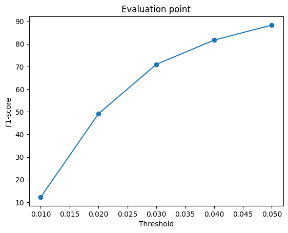
F1-scores across different threshold values.

Running Code Yourself

The source code can be found here. Please first download the dataset r2n2_shapenet_dataset 2.zip from here and uncompress the zip file.

Acknowledgment: This post has been inspired by the content from the course “Learning for 3D Vision” taught by Shubham Tulsiani at Carnegie Mellon University.

References:

• A Point Set Generation Network for 3D Object Reconstruction from a Single Image
• How to Optimize Data Transfers in CUDA C/C++
• TypeError: Cannot handle this data type: (1, 1, 3), <f4
• Deform a source mesh to form a target mesh using 3D loss functions