Profile ProcessQueue Class

8 minute read

It evaluates the performance of the ProcessQueue implementation from the previous post in terms of memory usage and CPU runtime.

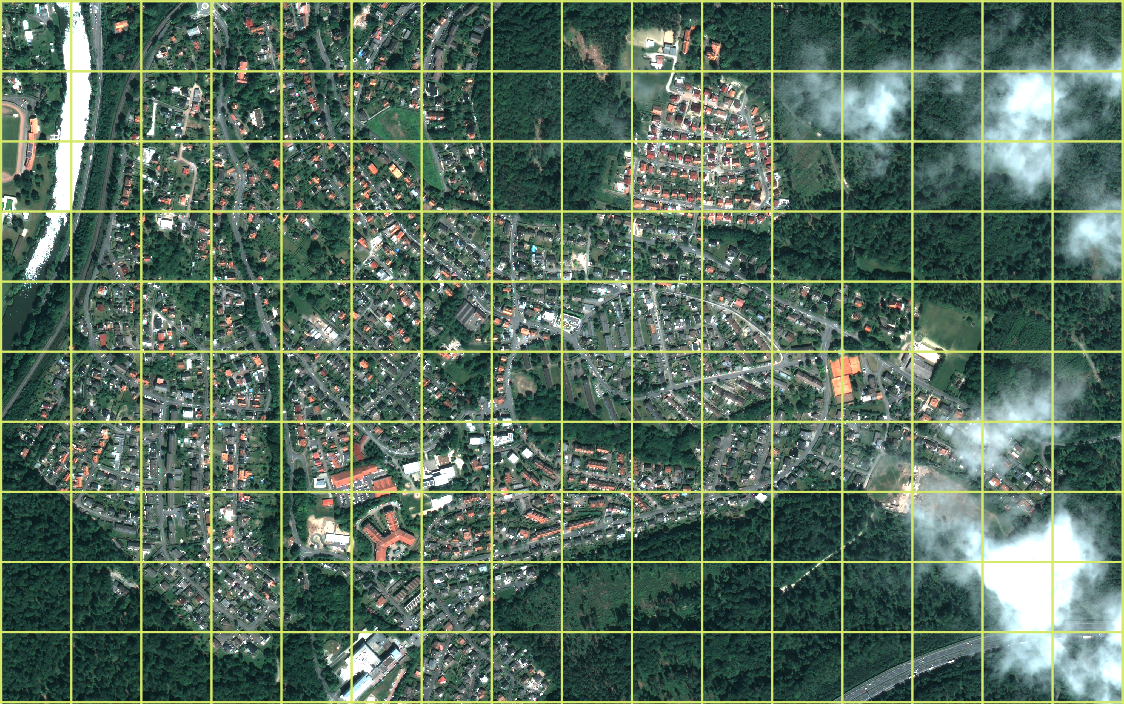
Figure: Satellite image after normalization by windows.

Introduction

In the previous post, a generic class ProcessQueue with Producer-Consumer pattern is implemented. In this post, I will profile a raster-processing program employing ProcessQueue concerning CPU and memory efficiency.

Satellite Imagery Multiprocessing

Being a geospatial software engineer, processing satellite imagery (also known as raster) has been one of the main tasks in my daily work. Usually, a raster file is the size of one to tens of gigabytes and is stored on a remote server. Thus, processing raster files could be considered both an IO- and CPU-intensive operation, which makes it perfect for showing the strength of ProcessQueue.

Processing by Windows

When working on a large raster file with the size of one to tens of gigabytes, it’s not realistic to read the whole raster into memory. Rasters’ data format GeoTiff allows users to read a part of the raster by specifying a window. The image below demonstrates how windows look overlapping the raster.

Windows are used to tile the raster/image.

Normalization Function

The task is to normalize rasters, which is done by the below function. Notice that I intentionally add the delay function as the previous post to mimic that a function takes longer to run in reality.

def normalize_image(image):
    # Make this function take longer to run.
    tmp = randint(1e5, 1e6)
    while tmp != 0:
        tmp -= 1

    image_ls = []
    for band in range(image.shape[0]):
        original_img = image[band, :, :]
        out_image = cv2.normalize(
            src=original_img,
            dst=None,
            alpha=0,
            beta=4096,
            norm_type=cv2.NORM_MINMAX,
            dtype=cv2.CV_16U,
        )
        image_ls.append(out_image)

    result = np.moveaxis(np.dstack(image_ls), 2, 0).astype(np.int64)
    return result

The normalized raster is shown below along with the original raster.

Figure: The bottom half of the image is original, and the top half of the image is normalized.

Glue Pieces Together

The main goal of this post is to show how a raster multiprocessing program works with queue and without queue. Therefore, two functions run_process_with_queue() and run_process_without_queue are created:

Processing with Queue

class ThreadQueue(threading.Thread):
    def __init__(self, in_queue, out_queue, fn: Callable):
        super().__init__()
        self.fn = fn
        self.in_queue = in_queue
        self.out_queue = out_queue

    def run(self):
        while True:
            data = self.in_queue.get()
            if isinstance(data, EndOfQueue):
                break
            result = self.fn(**data)
            self.out_queue.put(result)

def run_process_with_queue(input_path, output_path, num_processing_process):
    input_queue = multiprocessing.Manager().Queue(maxsize=20)
    output_queue = multiprocessing.Manager().Queue()
    ret_value_queue = multiprocessing.Manager().Queue()

    with open_raster(image_path=input_path, mode="r") as input_dataset:
        windows = [
            window for window in get_windows(dataset=input_dataset, window_size=256)
        ]

        print(f"Total windows: {len(windows)}")

        output_profile = copy.deepcopy(input_dataset.profile)

        reading_thread = threading.Thread(
            target=read_raster,
            args=(input_queue, input_dataset, windows),
        )

        processing_process = []
        for _ in range(num_processing_process):
            processing_process.append(
                ProcessQueue(
                    in_queue=input_queue,
                    out_queue=output_queue,
                    fn=(
                        lambda image, window: {
                            "image": normalize_image(image=image),
                            "window": window,
                        }
                    ),
                )
            )

        with open_raster(output_path, mode="w", **output_profile) as output_dataset:
            writing_thread = ThreadQueue(
                in_queue=output_queue,
                out_queue=ret_value_queue,
                fn=partial(write_raster, dataset=output_dataset),
            )

            for process in processing_process:
                process.daemon = True
                process.start()
            reading_thread.daemon = True
            reading_thread.start()
            writing_thread.daemon = True
            writing_thread.start()

            reading_thread.join()
            for _ in range(num_processing_process):
                input_queue.put(EndOfQueue())
            print("Reading is finished.")

            for process in processing_process:
                process.join()
            print("Processing is finished.")
            output_queue.put(EndOfQueue())

            writing_thread.join()
            print("Writing is finished.")

A new class ThreadQueue, which is similar to ProcessQueue, inherits threading.Thread and overrides run. ThreadQueue is used to spawn reading and writing threads, which read/write from/to data. Threads are used to fulfil IO-bound operations, as explained here. run_process_with_queue(input_path, output_path) connects the componenets together.

Here is a diagram depicting how each component assembles the whole pipeline. Note that the operations of reading, processing and writing happen simultaneously.

Figure: One thread reads data. Multiple processes process data. Another thread writes data. Note that reading and writing threads are spawned and are running in the main process.

Processing without Queue

Implementing multiprocessing without queue is more straightforward than with queue by reading the whole raster into memory in advance and then starting the data multiprocessing.

def run_process_without_queue(input_path, output_path, num_processing_process):
    with open_raster(image_path=input_path, mode="r") as input_dataset:
        windows = [
            window for window in get_windows(dataset=input_dataset, window_size=256)
        ]

        print(f"Total windows: {len(windows)}")

        output_profile = copy.deepcopy(input_dataset.profile)
        input_images = [input_dataset.read(window=window) for window in windows]
        print("Reading is finished.")

        with open_raster(output_path, mode="w", **output_profile) as output_dataset:
            with concurrent.futures.ProcessPoolExecutor(
                max_workers=num_processing_process
            ) as executor:
                for window, image in zip(
                    windows, executor.map(sharpen_image, input_images)
                ):
                    output_dataset.write(image, window=window)

Figure: The flow chart of multiprocessing without queue. The blue box indicates these events happen sequentially. First, it reads the data into memory. Second, it spawns child processes to process data and then writes data to files. Note that the processing and writing happen simultaneously.

Does using queue reduce processing time?

In the previous post, I discussed the scalability of the program. Let’s do it again here. The table below shows the program’s running time using different numbers of CPUs along with and without queue.

Num of CPUs	Running Time (sec): With Queue	Running Time (sec): Without Queue
2	31.5	29.3
4	20.4	21.9
8	18.6	19.0
16	17.9	18.7

The running time decreases when the number of CPUs increases. Even though it’s not perfect linear time reduction, it’s enough to show this program is scalable.
The required time to process this file can not be further decreased below 18 seconds.
In fact, if the delay function in normalize_image() is deleted, the processing time will be approximately 18 seconds, no matter whether the number of used CPUs is 2, 4, 8 or 16.
Due to above three reasons, we can conclude that this program is IO-bound. I.e., IO operation (reading and writing from/to files) requires more time than actually processing the data. Since the bottleneck is the IO operation, throwing more CPUs to this program only helps to reduce the running time to a certain extent. The last aside is that I intentionally add the delay function in normalize_image() only to show the scalability of this program.

Through this experiment, I learn that using queue does not reduce the actual processing time of data but the running time of a program. The analogy goes like this: let’s imagine it takes ten workers and ten days to build a house. Given the fixed number of workers, is it possible to make the construction time less than ten days? Apparently, the answer is no. No matter what software engineering trick is used, the amount of work is the same, the number of workers is the same, and it’s just impossible to build a house in less than ten days. It implies that if we want to use queue in our multiprocessing or multithreading program to decrease the processing time, it’s the wrong aim. However, using queue can reduce the running time of a program if this program involves heavy IO operations, as explained in the next section.

CPU and Memory Efficiency

I would like to demonstrate that using queue can indeed make a IO-intensive program run faster and be more memory efficient. The cloud platform, EC2 and S3 of AWS, and data are chosen as follow:

The EC2 instance m5.4xlarge (16 vCPUs and 64 GiB of momory) is used to run the experiment.
The data is stored on both EC2 and S3 bucket.
The size of the satellite image (GeoTiff) is 8.7 gigabytes. The raster must be tiled and pixel-interleave because reading band-interleave rasters from S3 is slower than reading pixel-interleave rasters from S3. If reading data is too slow in this experiment, the same bottleneck in the previous section will emerge.

The results are the following: the first table shows the memory usage in gigabytes (GBs), and the second table shows how much time it takes to run in seconds.

The function resource.getrusage(resource.RUSAGE_SELF).ru_maxrss is used in the main process to acquire the memory usage. The number in parenthesis is acquired by running Linux htop command while executing the program.

Memory Usage (Gigabytes):

Num of CPUs	With Queue Data on EC2	With Queue Data on S3	Without Queue Data on EC2	Without Queue Data on S3
2	3.5	3.5	13.1	13.1
4	3.5	3.5	13.1	13.1 (16.5)
8	3.5 (5.6)	3.5	13.1 (16.5)	13.1 (16.5)
16	3.5 (25.7)	3.5	13.1 (16.5)	13.1 (16.5)

Running Time of Program (Seconds):

Num of CPUs	With Queue Data on EC2	With Queue Data on S3	Without Queue Data on EC2	Without Queue Data on S3
2	610.7	1020.5	603.1	1600.2
4	210.3	1043.2	214.9	1228.6
8	131.8	982.2	106.3	1138.5
16	144.8	953.5	93.3	1111.9

As the previous section states, using queue can not reduce the processing time of the task. Let’s now move the environment to cloud and approach this task from memory and transferring speed perspective.

Experiments are conducted with different numbers of CPUs, and data is put on EC2 and S3 to show the effects of transferring speed in program’s running time. We can observe:

When using queue, memory usage is low as opposed to reading the whole data into memory in advance.
Spawning processes is expensive in Python.
Reading data from EC2 is much faster than reading data from S3. It takes 800 to 1000 seconds to read an eight gigabytes raster into memory by windows. One interesting aside is that it only takes less than one minute to transfer an eight gigabytes file from EC2 to S3. It teaches me that reading files into data structures is expensive, even if transferring speed is fast. The takeaway message is always transferring files from S3 to EC2, EBS, or EFS first, processing it and then deleting it, if possible. It will save a lot of reading time.
Using queue can help to reduce a program’s running time because a program starts processing data already when there is data read into queue if this program reads data from S3 directly. However, this phenomenon becomes less significant when the number of used CPUs grows. Again, the bottleneck of this program is the time it requires to read data from S3 but not the time it needs to process data.

Concatenation of two processing functions

The last aside is that we can concatenate two processing functions sequentially. For example, we can first normalize and sharpen an image:

def sharpen_image(image: np.ndarray):
    gaussian = np.array(
        [
            [1, 4, 7, 4, 1],
            [4, 16, 26, 16, 4],
            [7, 26, 41, 26, 7],
            [4, 16, 26, 16, 4],
            [1, 4, 7, 4, 1],
        ]
    )
    gaussian = gaussian / gaussian.sum()
    original = np.array(
        [
            [0, 0, 0, 0, 0],
            [0, 0, 0, 0, 0],
            [0, 0, 1, 0, 0],
            [0, 0, 0, 0, 0],
            [0, 0, 0, 0, 0],
        ]
    )

    # Due to associative property, do all multiplication on kernels as opposed
    # to image.
    sharpen_kernel = 2 * original - gaussian
    # Sharpen image twice.
    sharpen_kernel *= 2

    image_ls = []
    for band in range(image.shape[0]):
        image_ls.append(
            cv2.filter2D(src=image[band, :, :], ddepth=-1, kernel=sharpen_kernel)
        )
    result = np.moveaxis(np.dstack(image_ls), 2, 0).astype(np.int64)
    return result

normalized_image = normalize_image(image)
sharpened_image = sharpen_image(normalized_image)

Share on

Twitter Facebook LinkedIn