Using k-d tree to Find Holes with Various Sizes

Introduction

In the fascinating world of 3D computer vision, we often find ourselves dealing with 3D data like point clouds or their quirky cousins, 2.5D data, such as height models or depth maps. But, alas, the real world is rarely perfect, and our data can be quite unpredictable. Sometimes it’s noisy, other times it’s got more holes than Swiss cheese.

Today, we’re diving into how to use a k-d tree to deal with those holes in our 2D and 3D data. Let’s take a satellite stereo imagery pair as an example. A disparity map, shown below, is generated from satellite stereo imagery. We can observe that disparity values range from negative to positive due to the rectification process. (for those curious about stereo rectification and stereo matching, you can explore the notebooks here.)

Now, because of the quirks of stereo matching – occlusions, imperfect point correspondences, and just general mischief – this disparity map looks like it’s been to a cheese-tasting party. It’s got small holes, big holes, and everything in between. Those three big craters in the bottom-right corner? Blame it on the water bodies. They’re like the black holes of satellite imagery, devoid of texture and stumping the stereo matching algorithm.

So, here’s the deal: We want to sprinkle a little interpolation magic on our disparity map to fill those small holes, but we’re leaving the big holes to fend for themselves. Why, you ask? Because if we fill those big holes, it’s like telling our 3D point cloud generation buddies that everything’s peachy. It’s better to let them see the gaps and deal with them in their own unique way. We wouldn’t want them to get deceived by the interpolated holes, thinking there’s valuable data where there’s just emptiness.

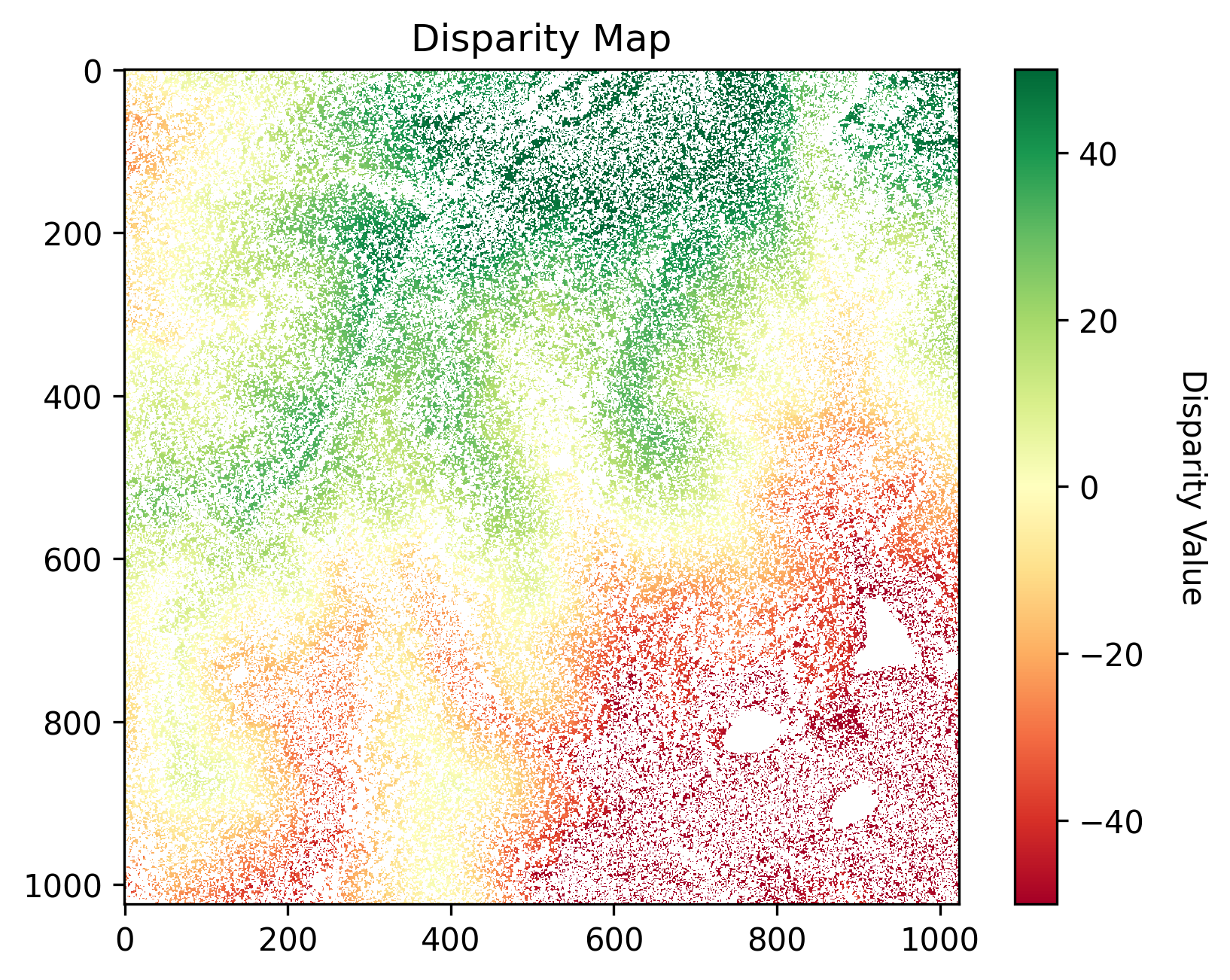
Raw disparity map acquired from stereo matching.

Using k-d Trees for Hole Detection

Understanding what a k-d tree does is as simple as looking at the following example. Consider an 8x8 array like this:

1 1 1 1 1 1 1 1
1 1 1 1 1 1 0 1
1 0 0 0 1 1 1 1
1 0 0 0 1 1 1 1
1 0 0 0 1 1 1 1
1 1 1 1 1 1 1 1
1 1 1 1 1 1 1 1
1 1 1 1 1 1 1 1

In this array, we want to identify the 0 at (2, 7) as a small hole and the 3x3 0 matrix as a big hole. In this article, I won’t explain how to construct a k-d tree; instead, I’ll show you how to use a k-d tree to solve this problem. The concept is straightforward: a k-d tree can help us find the nearest 1 to a target point 0. Once we identify the nearest neighbor 1, we can measure the distance between the 1 and 0. If the distance is smaller than a certain threshold, we consider the target point 0 to be a small hole. If it’s larger than the threshold, we classify it as a water body. Here’s a code snippet that accomplishes this:

def excluding_mesh(x, y, nan_x, nan_y, threshold):
    """Use KDTree to answer the question:
    Which point of set (x,y) is the nearest neighbors of those in (nan_x, nan_y)"""
    tree = cKDTree(np.c_[x, y])
    dist, j = tree.query(np.c_[nan_x, nan_y], k=1)

    # Select points sufficiently far away
    m = dist > threshold
    return nan_x[m], nan_y[m]

As a side note, we prefer to use cKDTree over KDTree because it’s significantly faster, a fact confirmed by many users.

The image below displays a binary mask generated using the code above. It highlights the large water bodies singled out by the k-d tree.

The binary mask reveals the locations of the large empty spaces.

Interpolating the Disparity Map

Once we’ve correctly identified the water bodies, the next step is to interpolate the disparity map and then apply a mask, as depicted in the image below.

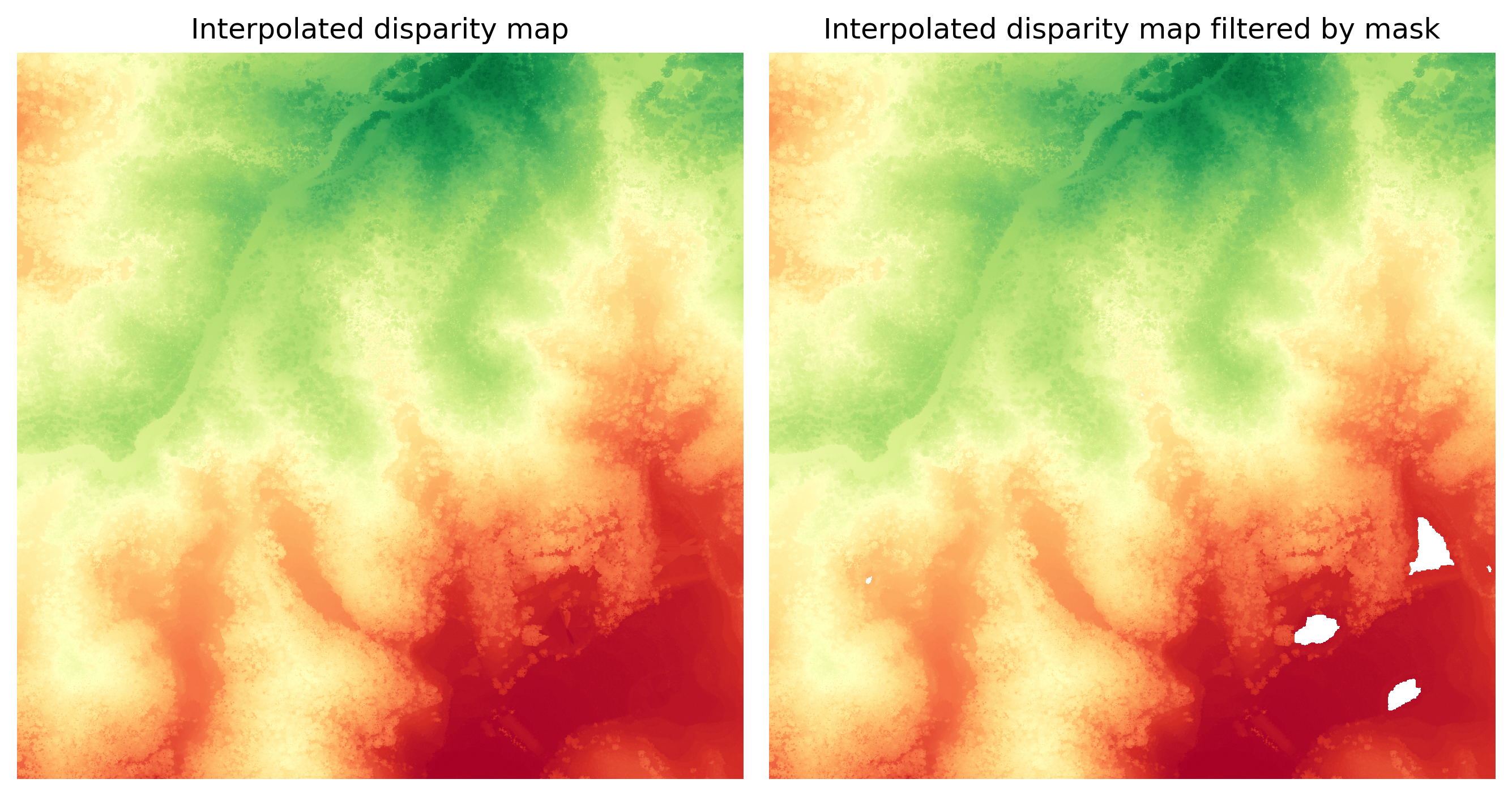
The image on the right retains well-interpolated pixels while excluding the water bodies.

And that’s it! In this article, we’ve demonstrated how to utilize a k-d tree to identify holes of various sizes in 2D data. This technique can easily be extended to the 3D realm, such as when you need to locate outliers in your 3D point clouds.

If you’d like to access the complete code used to generate the results in this post, it’s provided below.

from PIL import Image
import numpy as np
from scipy.interpolate import griddata
from scipy.spatial import KDTree, cKDTree
import matplotlib.pyplot as plt
import rasterio


def create_png_from_raster(raster_file_path):
    NODATA = -999.0
    with rasterio.open(raster_file_path) as src:
        arr = src.read()

    # arr[arr==src.nodata] = np.nan Not working bcs src.nodata is not set.
    arr[arr == NODATA] = np.nan
    # Make it more presentable.
    arr[arr >= 50] = 50
    arr[arr <= -50] = -50

    fig, ax = plt.subplots()
    ax.set_title(f"Disparity Map")
    im = ax.imshow(arr[0, :, :], cmap="RdYlGn")
    cbar = plt.colorbar(im)  # Add colorbar for reference
    cbar.set_label("Disparity Value", rotation=270, labelpad=20)
    # Save the figure as an image
    plt.savefig("disp_raw.png", dpi=300, bbox_inches="tight")


create_png_from_raster("disp_raw.tiff")


def excluding_mesh(x, y, nan_x, nan_y, threshold):
    """Use KDTree to answer the question:
    Which point of set (x,y) is the nearest neighbors of those in (nan_x, nan_y)"""
    tree = cKDTree(np.c_[x, y])
    dist, j = tree.query(np.c_[nan_x, nan_y], k=1)

    # Select points sufficiently far away
    m = dist > threshold
    return nan_x[m], nan_y[m]


def interpolate_array(arr: np.ndarray, method: str = "linear"):
    [n_rows, n_cols] = arr.shape
    print(f"Dimension (height, width): {n_rows} {n_cols}")

    # A meshgrid of pixel coordinates
    X, Y = np.meshgrid(np.arange(0, n_cols, 1), np.arange(0, n_rows, 1))

    # Find out finite values
    finite_idx = np.argwhere(np.isfinite(arr))
    if finite_idx.shape[0] == 0:
        # There is no finite value in arr.
        out = np.zeros((arr.shape))
    else:
        # Interpolate nan value. and fill convex hull with NAN.
        out = griddata(
            points=(finite_idx[:, 0], finite_idx[:, 1]),
            values=arr[finite_idx[:, 0], finite_idx[:, 1]],
            xi=(Y, X),
            method=method,
            fill_value=np.nan,
        )
    # Check the finite value in out.shape is the same as arr.shape
    # which means all value in out are finite.
    assert np.argwhere(np.isfinite(out)).shape[0] == arr.shape[0] * arr.shape[1]
    return out.astype(np.float32)


NODATA_VALUE = -999.0

disp_fname = "./disp_raw.tiff"

with Image.open(disp_fname) as im:
    disp = np.array(im).astype(np.float32)  # H x W

disp[disp == NODATA_VALUE] = np.nan

finite_idx = np.argwhere(np.isfinite(disp))
finite_idx_y = finite_idx[:, 0]
finite_idx_x = finite_idx[:, 1]

nan_idx = np.argwhere(np.isnan(disp))
nan_idx_y = nan_idx[:, 0]
nan_idx_x = nan_idx[:, 1]

xp, yp = excluding_mesh(finite_idx_x, finite_idx_y, nan_idx_x, nan_idx_y, threshold=5)
mask = np.zeros_like(disp).astype(np.uint8)

mask[yp, xp] = 1

plt.imsave("mask.png", mask, cmap="gray")

fig, ax = plt.subplots(nrows=1, ncols=2, figsize=(9, 6))
ax[0].set_title("Interpolated disparity map")
ax[1].set_title("Interpolated disparity map filtered by mask")
ax[0].set_axis_off()
ax[1].set_axis_off()

interpolated_arr = interpolate_array(arr=disp, method="nearest")
im = ax[0].imshow(interpolated_arr[:, :], cmap="RdYlGn")

assert np.isfinite(interpolated_arr).all() and mask.shape == interpolated_arr.shape

interpolated_arr[mask == 1] = np.nan

im = ax[1].imshow(interpolated_arr[:, :], cmap="RdYlGn")
fig.tight_layout()
plt.savefig("disp_itrpl.png", dpi=300, bbox_inches="tight")