Anatomy of NeRF, Neural Radiance Field

Neural Radiance Fields (NeRF) have emerged as a revolutionary approach to computer graphics and vision for synthesizing highly realistic images from sparse sets of images. At its core, NeRF models the continuous volumetric scene function using a multi-layer perceptron (MLP), mapping spatial coordinates and viewing directions to color and density. In this tutorial, I aim to demystify NeRF, explaining NeRF in detail and implementing it using PyTorch from the ground up by following [1].

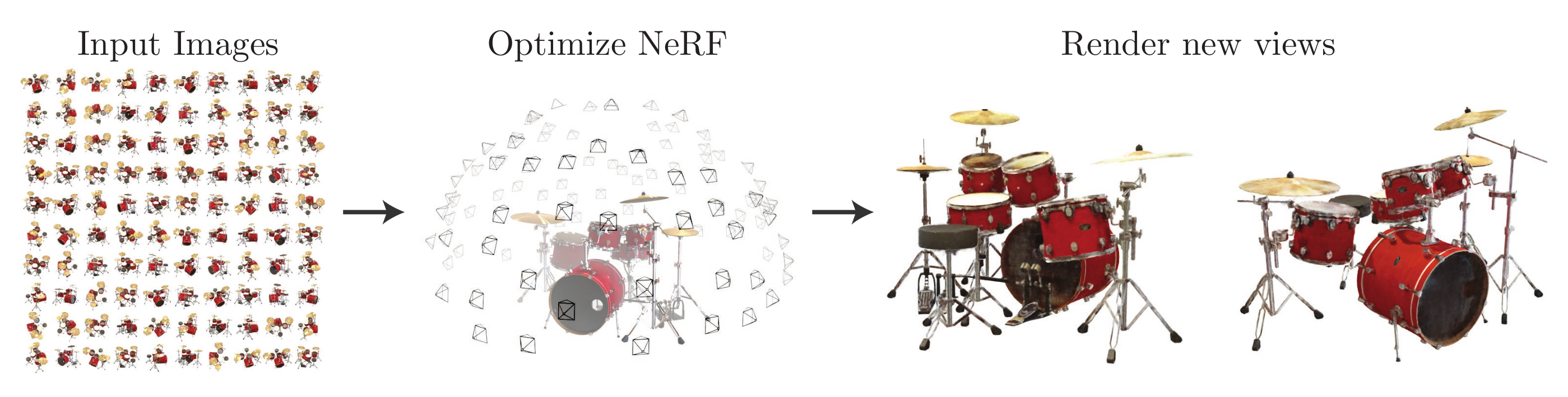
The sequence on the left illustrates the training images used for training a NeRF model, whereas the imagery on the right showcases the inference result.

References:

• [1] NeRF: Representing Scenes as Neural Radiance Fields for View Synthesis

Introduction

Neural Radiance Fields (NeRF) use a Multilayer Perceptron (MLP) network, represented by $F_{\Theta}$, where $\Theta$ denotes the network’s weights, to approximate a scene as a continuous 5D function. It does so by mapping a 5D vector, which includes a 3D spatial coordinate $\mathbf{x} = (x, y, z)$ and a 2D viewing direction $(\theta, \phi)$, to its associated volume density $\sigma$ and directional emitted color $\mathbf{c} = (r, g, b)$. Typically, the viewing direction is represented as a normalized 3D Cartesian vector $\mathbf{d}$.

An overview of NeRF. The image is adapted from [1].

The above visualization depicts the essence of NeRF. Training involves input images coupled with corresponding pose data, a spatial coordinate $\mathbf{x}$ and viewing direction $\mathbf{d}$, to refine an MLP. For rendering a new viewpoint, we only need to specify a pose information. The MLP then discerns the color for the input ray. Essentially, NeRF encodes the 3D scene within its MLP.

Volume Rendering with Radiance Fields

NeRF encapsulates a scene by capturing both the volume density $\sigma(\mathbf{x})$ and the directional emitted radiance at every spatial point. In this framework, $\sigma(\mathbf{x})$ represents the differential probability of a light ray being absorbed by an infinitesimally small particle at location $\mathbf{x}$. The expected color $C(\mathbf{r})$ for a camera ray $\mathbf{r}(t) = \mathbf{o} + t\mathbf{d}$, confined within the bounds $t_n$ and $t_f$, is calculated as:

\[C(\mathbf{r}) = \int_{t_n}^{t_f} T(t)\sigma(\mathbf{r}(t))\mathbf{c}(\mathbf{r}(t), \mathbf{d})dt, \quad \text{where} \quad T(t) = \exp \left( -\int_{t_n}^{t} \sigma(\mathbf{r}(s))ds \right).\]

The elements of this equation are explained as follows:

• $t$: the parameter along the ray, indicating the distance from the origin of the ray $\mathbf{o}$ to a point on its trajectory.
• $C(\mathbf{r})$: the expected scalar color acquired by the camera ray, aggregated from the color contributions along the ray’s path.
• $\sigma(\mathbf{r}(t))$: the volume density at a point on the ray, signaling the probability of a ray encountering a particle at that location.
• $\mathbf{c}(\mathbf{r}(t), \mathbf{d})$: the emitted color in direction $\mathbf{d}$ from a point on the ray, influenced by both the point’s position and the viewing direction.
• $T(t)$: the cumulative transmittance along the ray from $t_n$ to $t$, signifying the likelihood that the ray progresses from $t_n$ to $t$ without intersecting other particles.

To accurately evaluate the continuous integral $C(\mathbf{r})$ associated with each ray $\mathbf{r}$ emitting from the camera center, we can discretize the ray into a series of discrete segments. NeRF uses a stratified sampling which divides the interval $[t_n, t_f]$—which represents the segment of the ray being considered—into $N$ equally spaced intervals or bins. Within each bin, a sample point $t_i$ is chosen randomly, adhering to a uniform distribution. This process is mathematically expressed as follows:

\[t_i \sim U\left(t_n + \frac{(i - 1)}{N}(t_f - t_n), \, t_n + \frac{i}{N}(t_f - t_n)\right),\]

where $U(a, b)$ signifies a uniform distribution between $a$ and $b$, and $i$ varies from 1 to $N$, representing each discrete segment along the ray. The StratifiedRaysampler class below implements stratified sampling with slight modifications. Here, rays are discretized uniformly, and points are chosen uniformly, albeit deterministically. I found this approach is also effective as well.

class StratifiedRaysampler(torch.nn.Module):
    def __init__(self, n_pts_per_ray, min_depth, max_depth, **kwargs):
        super().__init__()

        self.n_pts_per_ray = n_pts_per_ray
        self.min_depth = min_depth
        self.max_depth = max_depth

    def forward(self, ray_bundle):
        # Compute z values for n_pts_per_ray points uniformly sampled between [near, far]
        z_vals = torch.linspace(
            start=self.min_depth, end=self.max_depth, steps=self.n_pts_per_ray
        ).to(ray_bundle.origins.device)
        z_vals = z_vals.view(
            1, -1, 1
        )  # Convert `torch.Size([n_pts_per_ray])` to `torch.Size([1, n_pts_per_ray, 1])`

        directions_view = ray_bundle.directions.view(
            -1, 1, 3
        )  # (num_rays, 3) -> (num_rays, 1, 3). No copy, just view.
        origins_view = ray_bundle.origins.view(
            -1, 1, 3
        )  # (num_rays, 3) -> (num_rays, 1, 3). No copy, just view.

        # Sample points from z values
        # (num_rays, n_pts_per_ray, 3) = (1, n_pts_per_ray, 1) * (num_rays, 1, 3) + (num_rays, 1, 3)
        sample_points = z_vals * directions_view + origins_view

        return ray_bundle._replace(
            sample_points=sample_points,
            sample_lengths=z_vals * torch.ones_like(sample_points[..., :1]),
        )

NeRF subsequently uses the samples $t_i$ to approximate $C(\mathbf{r})$ as follows:

\[\hat{C}(\mathbf{r}) = \sum_{i=1}^{N} T_i (1 - \exp(-\sigma_i \delta_i))\mathbf{c}_i, \quad \text{where} \quad T_i = \exp\left( -\sum_{j=1}^{i-1} \sigma_j \delta_j \right)\]

with $\delta_i = t_{i+1} - t_i$ denoting the distance between adjacent samples. This method for approximating $\hat{C}(\mathbf{r})$ from the set of $(\mathbf{c}_i, \sigma_i)$ values is inherently differentiable and simplifies to traditional alpha compositing, with alpha values $\alpha_i = 1 - \exp(-\sigma_i \delta_i)$. The methods _compute_weights and _aggregate within the VolumeRenderer class implements the functionality described above:

def _compute_weights(self, deltas, rays_density: torch.Tensor, eps: float = 1e-10):
    assert torch.all(deltas > 0)
    assert torch.all(rays_density >= 0)
    tmp_multiply = deltas * (rays_density)  # (num_rays, num_samples, 1)

    # Calculate the transmittance `T_i` along the ray for each sample point
    T_i = torch.exp(-torch.cumsum(tmp_multiply, dim=1)).to(rays_density.device)

    # Calculate weights `w_i` for each sample
    w_i = T_i * (1 - torch.exp(-tmp_multiply))  # FIXME: where is eps?
    return w_i

def _aggregate(self, weights: torch.Tensor, rays_feature: torch.Tensor):
    # Aggregate weighted sum of features using weights
    num_rays, num_samples, num_channel = rays_feature.shape
    assert weights.shape == (num_rays, num_samples, 1)

    feature = torch.sum(weights * rays_feature, dim=1)
    assert feature.shape == (num_rays, num_channel)
    return feature

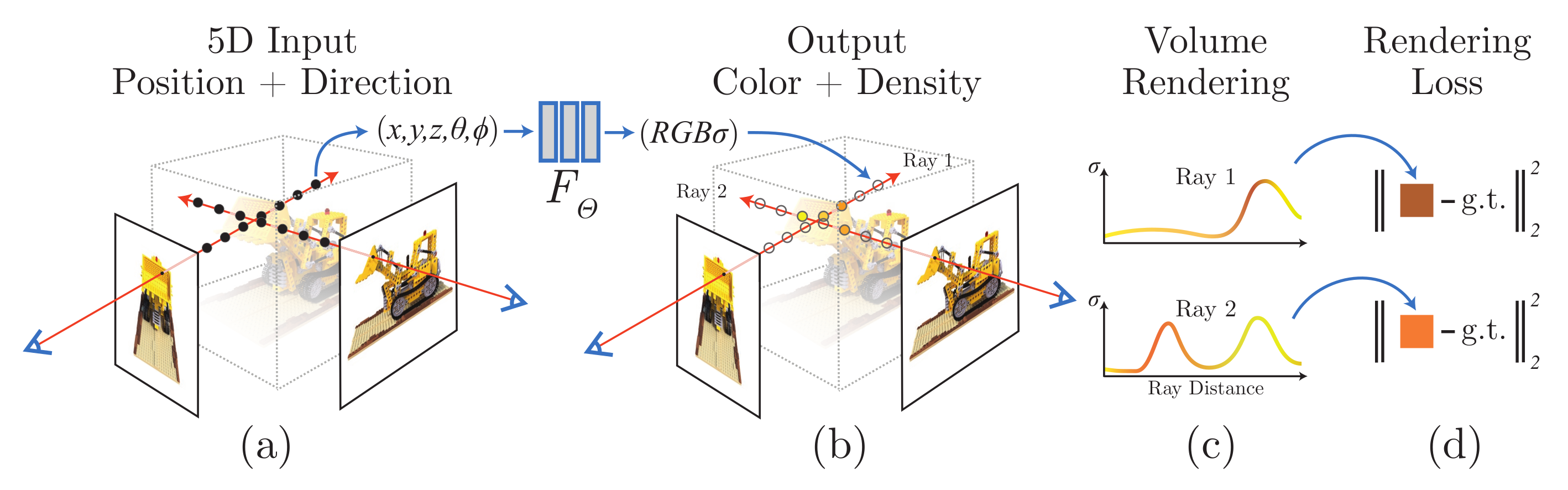
An overview of NeRF scene representation and differentiable rendering procedure. The image is adapted from [1].

The image above provides an overview of the NeRF scene representation and the differentiable rendering process. Panel (a) illustrates the sampling of 5D coordinates (comprising both location and viewing direction) along camera rays. Panel (b) demonstrates how these inputs are fed into an MLP to generate color and volume density. In (c), volume rendering techniques are applied to composite these outputs into an image (recall the meaning of $\hat{C}(\mathbf{r})$). This rendering process is inherently differentiable, enabling the optimization of the scene representation by minimizing the discrepancy between synthesized images and ground truth observations, as shown in (d).

Note: In traditional alpha compositing, alpha values range from 0 to 1, representing a pixel’s transparency level. An alpha of 1 indicates full opacity, while an alpha of 0 signifies complete transparency. In the context of NeRF, the alpha value is derived from the volume density $\sigma_i$ at a specific sample point and the distance $\delta_i$ to the subsequent sample along a ray. A higher product of $\sigma_i$ and $\delta_i$ implies a denser medium. Given that both $\sigma_i$ and $\delta_i$ are positive, the expression $\exp(-\sigma_i \delta_i)$ naturally falls within the [0, 1] range. Therefore, $\alpha_i = 1 - \exp(-\sigma_i \delta_i)$ effectively translates a greater combination of volume density and sample distance into increased alpha.

NeRF’s Model Architecture

The overall fully-connected network architecture of NeRF is shown below.

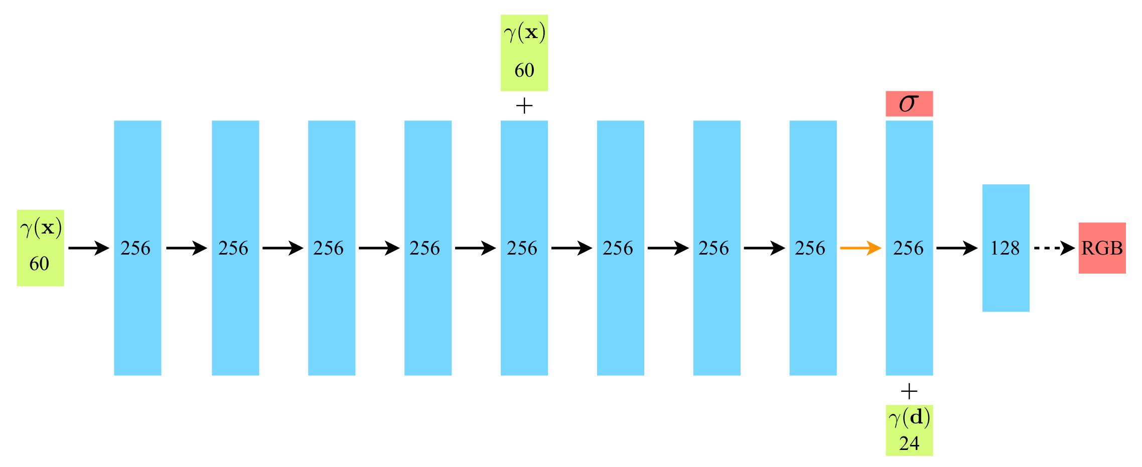
A visualization of NeRF's fully-connected network. The image is adapted from [1].

The architecture is detailed as follows: Inputs (green) flow through hidden layers (blue) to outputs (red), with block numbers indicating vector dimensions. It uses standard fully-connected layers composed of ReLU activations (black arrows), layers without activations (orange arrows), and sigmoid activations (dashed black arrows). Vector concatenation is represented by “+”. Positional encoding $\gamma(\mathbf{x})$ passes through eight 256-channel ReLU layers, including a skip connection at the fifth layer. Up to the point marked by the orange arrow, the model is encapsulated as MLPWithInputSkips, detailed below:

class MLPWithInputSkips(torch.nn.Module):
    """Implement Figure 7 from [Mildenhall et al. 2020], an MLP with a skip connection."""

    def __init__(
        self, n_layers, input_dim, output_dim, skip_dim, hidden_dim, input_skips
    ):
        super().__init__()
        self._input_skips = set(input_skips)

        layers = []
        for i in range(n_layers):
            # The first and last layer can also be skip layer.
            dimin = input_dim if i == 0 else hidden_dim  # first layer
            dimout = output_dim if i == n_layers - 1 else hidden_dim  # last layer
            if i in self._input_skips:
                dimin += skip_dim

            linear = torch.nn.Linear(dimin, dimout)

            if i < n_layers - 1:
                layers.append(torch.nn.Sequential(linear, torch.nn.ReLU(inplace=True)))
            elif i == n_layers - 1:  # Last layer has no activation
                layers.append(torch.nn.Sequential(linear))

        self._mlp = torch.nn.ModuleList(layers)

    def forward(self, x: torch.Tensor, skip_pos: torch.Tensor) -> torch.Tensor:
        # NOTE: Python is pass-by-reference, torch.Tensor is mutable and `ReLU(inplace=True)`.
        # Does the following code have any UNEXPEXTED side effect when `x is skip_pos`?
        # tmp_id = id(skip_pos)
        for i, layer in enumerate(self._mlp):
            if i in self._input_skips:
                x = torch.cat((x, skip_pos), dim=-1)
            x = layer(x)
        # assert tmp_id == id(skip_pos)
        return x

In forward, passing identical torch.Tensor v as both x and skip_pos, such as MLPWithInputSkips()(v, v), results in x and skip_pos sharing the same id as v. Despite using ReLU(inplace=True), x is not overwritten; instead, Python generates a new object for x at each x = layer(x) operation, preserving the original v and skip_pos. I am not sure how to explain this behaviour but record the result here.

Following the previous layers, a subsequent layer outputs non-negative volume density $\sigma$ (via ReLU) and a 256-dimensional feature vector. This vector, when concatenated with $\gamma(\mathbf{d})$, undergoes further processing by a 128-channel ReLU layer. A sigmoid-activated final layer outputs RGB radiance at $\mathbf{x}$ for direction $\mathbf{d}$. The NeuralRadianceField class implements this process as follows:

class NeuralRadianceField(torch.nn.Module):
    """Implement NeRF."""

    def __init__(self, cfg):
        super().__init__()
        self.harmonic_embedding_xyz = HarmonicEmbedding(3, cfg.n_harmonic_functions_xyz)
        self.harmonic_embedding_dir = HarmonicEmbedding(3, cfg.n_harmonic_functions_dir)

        embedding_dim_xyz = (
            self.harmonic_embedding_xyz.output_dim
        )  # 3 * n_harmonic_functions_xyz * 2
        embedding_dim_dir = (
            self.harmonic_embedding_dir.output_dim
        )  # 3 * n_harmonic_functions_dir * 2

        self.xyz_out_layer = MLPWithInputSkips(
            n_layers=cfg.n_layers_xyz,
            input_dim=embedding_dim_xyz,
            output_dim=cfg.n_hidden_neurons_xyz,
            skip_dim=embedding_dim_xyz,
            hidden_dim=cfg.n_hidden_neurons_xyz,
            input_skips=cfg.append_xyz,
        )
        self.density_out_layer = torch.nn.Sequential(
            torch.nn.Linear(cfg.n_hidden_neurons_xyz, 1),
            torch.nn.ReLU(inplace=True),  # ensure density being nonnegative
        )
        self.feature_vector = torch.nn.Sequential(
            torch.nn.Linear(cfg.n_hidden_neurons_xyz, cfg.n_hidden_neurons_xyz),
            torch.nn.ReLU(inplace=True),
        )

        self.rgb_out_layer = torch.nn.Sequential(
            torch.nn.Linear(
                embedding_dim_dir + cfg.n_hidden_neurons_xyz, cfg.n_hidden_neurons_dir
            ),
            torch.nn.ReLU(inplace=True),
            torch.nn.Linear(cfg.n_hidden_neurons_dir, 3),
            torch.nn.Sigmoid(),  # (r, g, b) in [0, 1]
        )

    def forward(self, ray_bundle):  # ray_bundle: (num_rays, )
        pos = ray_bundle.sample_points  # (num_rays, n_pts_per_ray, 3)
        dir = ray_bundle.directions  # (num_rays, 3)
        position_encoding = self.harmonic_embedding_xyz(pos)
        direction_encoding = self.harmonic_embedding_dir(dir)
        # tmp = position_encoding.clone()
        xyz_out = self.xyz_out_layer(position_encoding, position_encoding)
        # assert torch.equal(position_encoding, tmp)
        density = self.density_out_layer(xyz_out)
        feature = self.feature_vector(xyz_out)

        expanded_direction_encoding = direction_encoding.unsqueeze(1).repeat(
            1, feature.shape[1], 1
        )  # (num_rays, 24) --> (num_rays, 1, 24) --> (num_rays, n_pts_per_ray, 24)

        # Concatenate feature and expanded_direction_encoding
        rgb = self.rgb_out_layer(
            torch.cat([feature, expanded_direction_encoding], dim=-1)
        )

        return {"density": density, "feature": rgb}

The network outputs a dictionary comprising two components: a density value $\sigma$ and a feature vector representing color $\mathbf{c} = (r, g, b)$.

Position Encoding

According to [1], input coordinates undergo transformation into a higher-dimensional space through the function $\gamma$. This enhances the network’s capacity to capture high-frequency variations. The transformation $\gamma(p)$ for each coordinate is as follows:

\[\gamma(p) = (\sin(2^0 \pi p), \cos(2^0 \pi p), ..., \sin(2^{L-1} \pi p), \cos(2^{L-1} \pi p)).\]

The HarmonicEmbedding class implements the $\gamma(p)$ function, detailed as follows:

class HarmonicEmbedding(torch.nn.Module):
    """Implement position encoding in NeRF."""

    def __init__(
        self, in_channels: int = 3, n_harmonic_functions: int = 6, omega0: float = 1.0
    ) -> None:
        super().__init__()

        frequencies = 2.0 ** torch.arange(n_harmonic_functions, dtype=torch.float32)
        self.register_buffer("_frequencies", omega0 * frequencies, persistent=False)
        self.output_dim = n_harmonic_functions * 2 * in_channels

    def forward(self, x: torch.Tensor):
        embed = (x[..., None] * self._frequencies).view(*x.shape[:-1], -1)
        return torch.cat((embed.sin(), embed.cos()), dim=-1)

The function $\gamma(\cdot)$ is applied to each component of the spatial coordinates $\mathbf{x}$ and the Cartesian viewing direction vector $\mathbf{d}$, with both normalized within $[-1, 1]$. As specified in [1], $\gamma(\mathbf{x})$ uses $L=10$ and $\gamma(\mathbf{d})$ uses $L=4$. Consequently, given the calculations 3x10x2=60 for $\gamma(\mathbf{x})$ and 3x4x2=24 for $\gamma(\mathbf{d})$, these dimensions, 60 and 24 respectively, are illustrated in the model’s architectural diagram.

Hierarchical Volume Sampling

Work in progress.

Depth vs. Inverse-Depth Sampling

Work in progress.

Defining Loss

In [1], the method involves randomly sampling batches of camera rays from pixel data and applying hierarchical sampling to collect $N_c$ samples via a “coarse” network and $N_c + N_f$ samples through a “fine” network. As hierarchical volume sampling is currently under development, I will focus solely on the loss function excluding hierarchical volume sampling aspects. Hence, the loss is defined as the total squared error between the rendered colors from the coarse renderings and the actual pixel colors:

\[L = \sum_{\mathbf{r} \in R} \left( \| \hat{C}_c(\mathbf{r}) - C(\mathbf{r}) \|^2_2 \right),\]

where $R$ is the set of sampled rays, and $C(\mathbf{r})$ and $\hat{C}_c(\mathbf{r})$ denote the ground truth and coarse predicted colors for ray $\mathbf{r}$, respectively.

Experimentation Results

In this section, I evaluate my NeRF implementation using three datasets: “Lego”, “Fern”, and “Materials”. Below are visual representations of the training images from each dataset:

Training dataset.

Fern

Lego

Materials

To perform inference using NeRF, the model requires the camera’s position, $\mathbf{x}$, and the viewing direction, $\mathbf{d}$. The inference results for three datasets are shown below:

Inferencing with continuous viewing directions.

Fern

Lego

Materials

Discussion:

The initial results show that although it is feasible to extract a 3D model from the trained NeRF model, the rendering quality appears notably less sharp compared to the original training images. Here are several plausible explanations:

1. Lack of Hierarchical Volume Sampling: The absence of hierarchical volume sampling in my approach may result in insufficient resolution of detail.

2. Limited Training Duration: According to [1], optimal training of a NeRF model for each scene requires 1-2 days. In contrast, my models have been trained for merely a few hours (less than 10). Additionally, it appears that the training cost can continue to decrease, albeit at a very slow pace, if I were to continue training.

3. Constraints on Position and Viewing Direction: I observed that deviations in the camera’s position and viewing direction from those of the original training images affect rendering quality.

4. Dataset Limitations: The parts of the rendered scene not covered by the training images, such as the area surrounding the fern, exhibit noise.

Running Code Yourself

The source code can be found here.

The “materials” dataset can be downloaded here.

Acknowledgment: This post has been inspired by the content from the course “Learning for 3D Vision” taught by Shubham Tulsiani at Carnegie Mellon University.